Critical Value Calculator

Get the critical values associated with a particular significance level (alpha) and statistical distributions with the critical value calculator.

The calculator functions to provide left-tailed, right-tailed, and two-tailed P values for Chi-square, T, F, R, and Z score values that help you better judge the critical points of the given probability density function.

What Is a Critical Value?

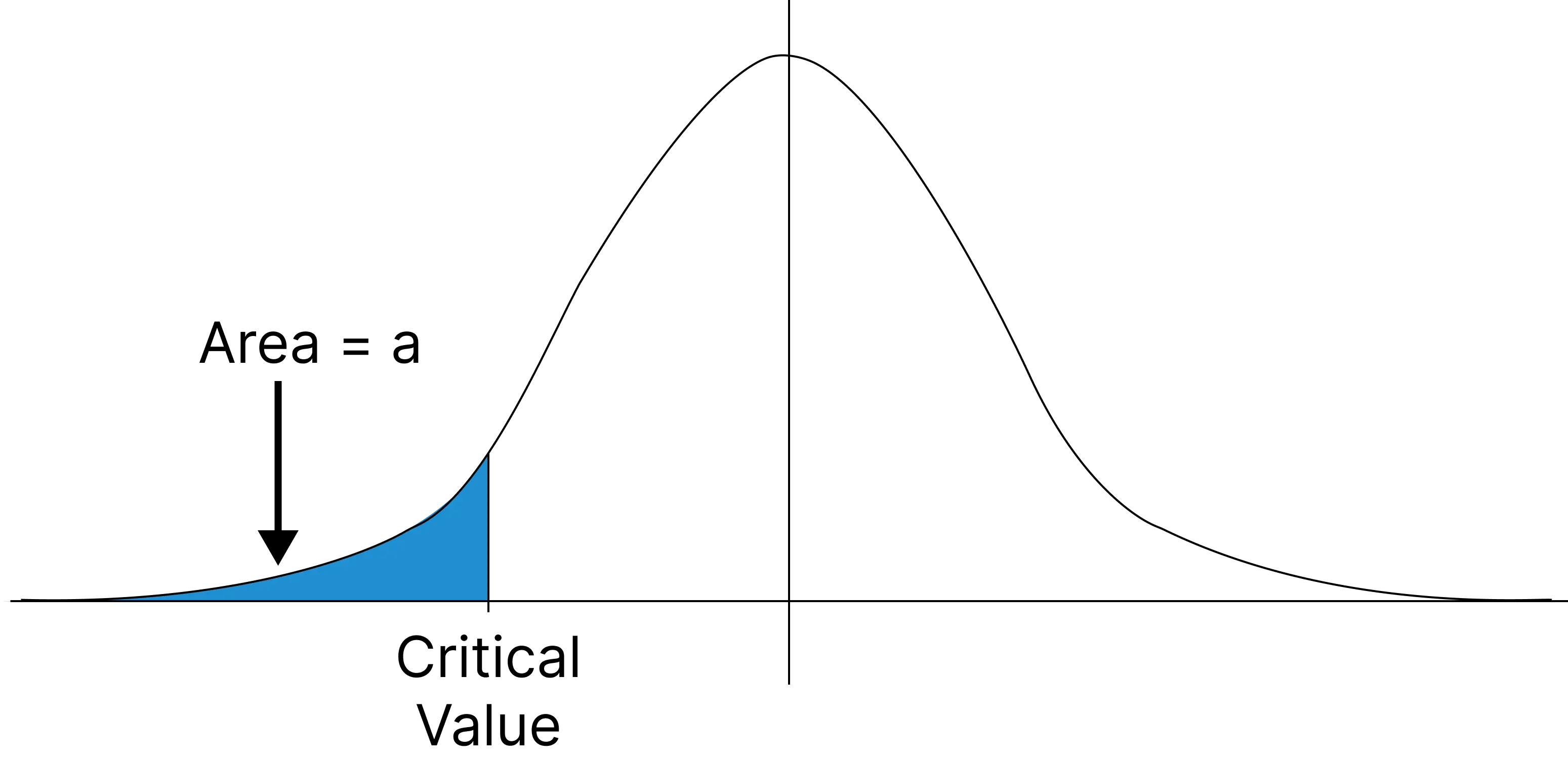
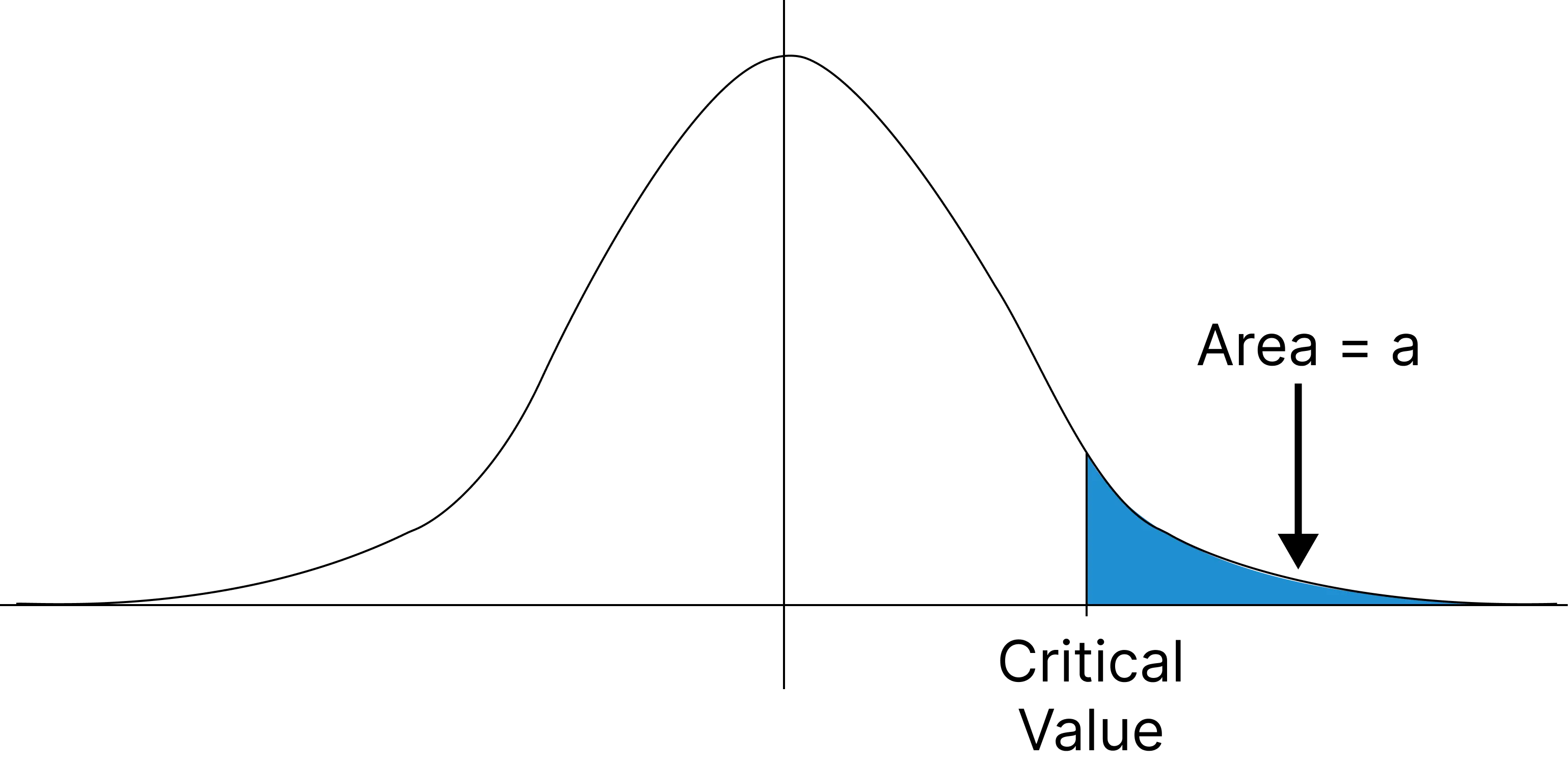
A critical value is said to be as a line on a graph that divides a distribution graph into sections that indicate ‘rejection regions.’ Generally, if a test value falls into a rejection rejoin, then it means that an accepted hypothesis (represent as a null hypothesis) should be rejected.

Left-tailed: Q (α)

left tailed

Right-tailed: Q (1 – α)

right tailed

Two-tailed: Q (α/2)] ∪ Q (1 – α/2)

two tailed

How to Calculate Critical Value With This Tool

Simply, you just have to follow the given steps:

Find Critical Value for T

Inputs:

At first, you ought to select the option “Critical value for t” from the drop-down list
Now, you just have to add the value of the “significance level” into the designated field
Finally, you have to add the value of “degrees of freedom” into the designated field

Outputs:

After adding values into the above fields, just hit the calculate button:

Critical value for t (Right Tailed)
Critical value for t (Two Tailed)

Find Critical Value For Z

Inputs:

You just have to choose the option “Critical value for z” form the drop-down menu of this tool
Right after, you ought to add the value of the “significance level” into the given box

Outputs:

Now, hit the calculate button, this z value calculator will show:

Critical value for z (Right Tailed)
Critical value for z (Two Tailed)

Find Critical Value for Chi-Square

Inputs:

First, choose the option “Critical value for chi-square” form the list of drop-down
Then, simply add the value for a “significance level” into the above-designated box
Very next, add the value for a “degrees of freedom” into the given field of calculator

Outputs:

Now, you have to make a click on the calculate button to calculate chi square value for the distribution, the tool generates:

Chi-Square critical value (Right Tailed)
Chi-Square critical value (Two Tailed)
P value (for the chi square distribution)

Find Critical Value For F

Inputs:

First, choose the option of “Critical value for f” from the given drop-down menu
Very next, you have to enter the value of a “degrees of freedom 1” into the designated field
Right after, you ought to add the value of a “degrees if freedom 2” into the given box
Finally, put the value of “significance level” into the designated box

Outputs:

Once done, click on the calculate button, this f value calculator will generate:

Critical value f (Right Tailed)
Critical value f (Two Tailed)

Z Score Table (Right):

The z-table is the normal distribution shows the area to the right-hand side of the curve. You can use these values to determine the area between z=0 and any positive (+) value.

z	0.00	0.01	0.02	0.03	0.04	0.05	0.06	0.07	0.08	0.09
0.0	0.0000	0.0040	0.0080	0.0120	0.0160	0.0199	0.0239	0.0279	0.0319	0.0359
0.1	0.0398	0.0438	0.0478	0.0517	0.0557	0.0596	0.0636	0.0675	0.0714	0.0753
0.2	0.0793	0.0832	0.0871	0.0910	0.0948	0.0987	0.1026	0.1064	0.1103	0.1141
0.3	0.1179	0.1217	0.1255	0.1293	0.1331	0.1368	0.1406	0.1443	0.1480	0.1517
0.4	0.1554	0.1591	0.1628	0.1664	0.1700	0.1736	0.1772	0.1808	0.1844	0.1879
0.5	0.1915	0.1950	0.1985	0.2019	0.2054	0.2088	0.2123	0.2157	0.2190	0.2224
0.6	0.2257	0.2291	0.2324	0.2357	0.2389	0.2422	0.2454	0.2486	0.2517	0.2549
0.7	0.2580	0.2611	0.2642	0.2673	0.2704	0.2734	0.2764	0.2794	0.2823	0.2852
0.8	0.2881	0.2910	0.2939	0.2967	0.2995	0.3023	0.3051	0.3078	0.3106	0.3133
0.9	0.3159	0.3186	0.3212	0.3238	0.3264	0.3289	0.3315	0.3340	0.3365	0.3389
1.0	0.3413	0.3438	0.3461	0.3485	0.3508	0.3531	0.3554	0.3577	0.3599	0.3621
1.1	0.3643	0.3665	0.3686	0.3708	0.3729	0.3749	0.3770	0.3790	0.3810	0.3830
1.2	0.3849	0.3869	0.3888	0.3907	0.3925	0.3944	0.3962	0.3980	0.3997	0.4015
1.3	0.4032	0.4049	0.4066	0.4082	0.4099	0.4115	0.4131	0.4147	0.4162	0.4177
1.4	0.4192	0.4207	0.4222	0.4236	0.4251	0.4265	0.4279	0.4292	0.4306	0.4319
1.5	0.4332	0.4345	0.4357	0.4370	0.4382	0.4394	0.4406	0.4418	0.4429	0.4441
1.6	0.4452	0.4463	0.4474	0.4484	0.4495	0.4505	0.4515	0.4525	0.4535	0.4545
1.7	0.4554	0.4564	0.4573	0.4582	0.4591	0.4599	0.4608	0.4616	0.4625	0.4633
1.8	0.4641	0.4649	0.4656	0.4664	0.4671	0.4678	0.4686	0.4693	0.4699	0.4706
1.9	0.4713	0.4719	0.4726	0.4732	0.4738	0.4744	0.4750	0.4756	0.4761	0.4767
2.0	0.4772	0.4778	0.4783	0.4788	0.4793	0.4798	0.4803	0.4808	0.4812	0.4817
2.1	0.4821	0.4826	0.4830	0.4834	0.4838	0.4842	0.4846	0.4850	0.4854	0.4857
2.2	0.4861	0.4864	0.4868	0.4871	0.4875	0.4878	0.4881	0.4884	0.4887	0.4890
2.3	0.4893	0.4896	0.4898	0.4901	0.4904	0.4906	0.4909	0.4911	0.4913	0.4916
2.4	0.4918	0.4920	0.4922	0.4925	0.4927	0.4929	0.4931	0.4932	0.4934	0.4936
2.5	0.4938	0.4940	0.4941	0.4943	0.4945	0.4946	0.4948	0.4949	0.4951	0.4952
2.6	0.4953	0.4955	0.4956	0.4957	0.4959	0.4960	0.4961	0.4962	0.4963	0.4964
2.7	0.4965	0.4966	0.4967	0.4968	0.4969	0.4970	0.4971	0.4972	0.4973	0.4974
2.8	0.4974	0.4975	0.4976	0.4977	0.4977	0.4978	0.4979	0.4979	0.4980	0.4981
2.9	0.4981	0.4982	0.4982	0.4983	0.4984	0.4984	0.4985	0.4985	0.4986	0.4986
3.0	0.4987	0.4987	0.4987	0.4988	0.4988	0.4989	0.4989	0.4989	0.4990	0.4990
3.1	0.4990	0.4991	0.4991	0.4991	0.4992	0.4992	0.4992	0.4992	0.4993	0.4993
3.2	0.4993	0.4993	0.4994	0.4994	0.4994	0.4994	0.4994	0.4995	0.4995	0.4995
3.3	0.4995	0.4995	0.4995	0.4996	0.4996	0.4996	0.4996	0.4996	0.4996	0.4997
3.4	0.4997	0.4997	0.4997	0.4997	0.4997	0.4997	0.4997	0.4997	0.4997	0.4998
3.5	0.4998	0.4998	0.4998	0.4998	0.4998	0.4998	0.4998	0.4998	0.4998	0.4998
3.6	0.4998	0.4998	0.4999	0.4999	0.4999	0.4999	0.4999	0.4999	0.4999	0.4999
3.7	0.4999	0.4999	0.4999	0.4999	0.4999	0.4999	0.4999	0.4999	0.4999	0.4999
3.8	0.4999	0.4999	0.4999	0.4999	0.4999	0.4999	0.4999	0.4999	0.4999	0.4999

Z Score Table (Left):

The left z-table shows the area to the left of Z.

Z	0.00	0.01	0.02	0.03	0.04	0.05	0.06	0.07	0.08	0.09
0.0	0.5000	0.5040	0.5080	0.0120	0.0160	0.0199	0.5239	0.0279	0.0319	0.0359
0.1	0.5398	0.5438	0.5478	0.5517	0.5557	0.5596	0.5636	0.5675	0.5714	0.5753
0.2	0.5793	0.5832	0.5871	0.5910	0.5948	0.5987	0.6064	0.1064	0.6103	0.6141
0.3	0.6179	0.6217	0.6255	0.6293	0.6331	0.6368	0.6406	0.6443	0.6480	0.6517
0.4	0.6554	0.6591	0.6628	0.6664	0.6700	0.6736	0.6772	0.6808	0.6844	0.6879
0.5	0.6915	0.6950	0.6985	0.7019	0.7054	0.7088	0.7123	0.7157	0.7190	0.7224
0.6	0.7257	0.7291	0.7324	0.7357	0.7389	0.7422	0.7454	0.7486	0.7517	0.7549
0.7	0.7580	0.7611	0.7642	0.7673	0.7704	0.7734	0.7764	0.7794	0.7823	0.7852
0.8	0.7881	0.7910	0.7939	0.7967	0.7995	0.8023	0.8051	0.8078	0.8106	0.8133
0.9	0.8159	0.8186	0.8212	0.8238	0.8264	0.8289	0.8315	0.8340	0.8365	0.8389
1.0	0.8413	0.8438	0.8461	0.8485	0.8508	0.8531	0.8554	0.8577	0.8599	0.8621
1.1	0.8643	0.8665	0.8686	0.8708	0.8729	0.8749	0.8770	0.8790	0.8810	0.8830
1.2	0.8849	0.8869	0.8888	0.8907	0.8925	0.8944	0.8962	0.8980	0.8997	0.9015
1.3	0.9032	0.9049	0.9066	0.9082	0.9099	0.9115	0.9131	0.9147	0.9162	0.9177
1.4	0.9192	0.9207	0.9222	0.9236	0.9251	0.9265	0.9279	0.9292	0.9306	0.9319
1.5	0.9332	0.9345	0.9357	0.9370	0.9382	0.9394	0.9406	0.9418	0.9429	0.9441
1.6	0.9452	0.9463	0.9474	0.9484	0.9495	0.9505	0.9515	0.9525	0.9535	0.9545
1.7	0.9554	0.9564	0.9573	0.9582	0.9591	0.9599	0.9608	0.9616	0.9625	0.9633
1.8	0.9641	0.9649	0.9656	0.9664	0.9671	0.9678	0.9686	0.9693	0.9699	0.9706
1.9	0.9713	0.9719	0.9726	0.9732	0.9738	0.9744	0.9750	0.9756	0.9761	0.9767
2.0	0.9772	0.9778	0.9783	0.9788	0.9793	0.9798	0.9803	0.9808	0.9812	0.9817
2.1	0.9821	0.9826	0.9830	0.9834	0.9838	0.9842	0.9846	0.9850	0.9854	0.9857
2.2	0.9861	0.9864	0.9868	0.9871	0.9875	0.9878	0.9881	0.9884	0.9887	0.9890
2.3	0.9893	0.9896	0.9898	0.9901	0.9904	0.9906	0.9909	0.9911	0.9913	0.9916
2.4	0.9918	0.9920	0.9922	0.9925	0.9927	0.9929	0.9931	0.9932	0.9934	0.9936
2.5	0.9938	0.9940	0.9941	0.9943	0.9945	0.9946	0.9948	0.9949	0.9951	0.9952
2.6	0.9953	0.9955	0.9956	0.9957	0.9959	0.9960	0.9961	0.9962	0.9963	0.9964
2.7	0.9965	0.9966	0.9967	0.9968	0.9969	0.9970	0.9971	0.9972	0.9973	0.9974
2.8	0.9974	0.9975	0.9976	0.9977	0.9977	0.9978	0.9979	0.9979	0.9980	0.9981
2.9	0.9981	0.9982	0.9982	0.9983	0.9984	0.9984	0.9985	0.9985	0.9986	0.9986
3.0	0.9987	0.9987	0.9987	0.9988	0.9988	0.9989	0.9989	0.9989	0.9990	0.9990

T Critical Value Table (One Tail):

df	a = 0.1	0.05	0.025	0.01	0.005	0.001	0.0005
∞	t_a = 1.282	1.645	1.960	2.326	2.576	3.091	3.291
1	3.078	6.314	12.706	31.821	63.656	318.289	636.578
2	1.886	2.920	4.303	6.965	9.925	22.328	31.600
3	1.638	2.353	3.182	4.541	5.841	10.214	12.924
4	1.533	2.132	2.776	3.747	4.604	7.173	8.610
5	1.476	2.015	2.571	3.365	4.032	5.894	6.869
6	1.440	1.943	2.447	3.143	3.707	5.208	5.959
7	1.415	1.895	2.365	2.998	3.499	4.785	5.408
8	1.397	1.860	2.306	2.896	3.355	4.501	5.041
9	1.383	1.833	2.262	2.821	3.250	4.297	4.781
10	1.372	1.812	2.228	2.764	3.169	4.144	4.587
11	1.363	1.796	2.201	2.718	3.106	4.025	4.437
12	1.356	1.782	2.179	2.681	3.055	3.930	4.318
13	1.350	1.771	2.160	2.650	3.012	3.852	4.221
14	1.345	1.761	2.145	2.624	2.977	3.787	4.140
15	1.341	1.753	2.131	2.602	2.947	3.733	4.073
16	1.337	1.746	2.120	2.583	2.921	3.686	4.015
17	1.333	1.740	2.110	2.567	2.898	3.646	3.965
18	1.330	1.734	2.101	2.552	2.878	3.610	3.922
19	1.328	1.729	2.093	2.539	2.861	3.579	3.883
20	1.325	1.725	2.086	2.528	2.845	3.552	3.850
21	1.323	1.721	2.080	2.518	2.831	3.527	3.819
22	1.321	1.717	2.074	2.508	2.819	3.505	3.792
23	1.319	1.714	2.069	2.500	2.807	3.485	3.768
24	1.318	1.711	2.064	2.492	2.797	3.467	3.745
25	1.316	1.708	2.060	2.485	2.787	3.450	3.725
26	1.315	1.706	2.056	2.479	2.779	3.435	3.707
27	1.314	1.703	2.052	2.473	2.771	3.421	3.689
28	1.313	1.701	2.048	2.467	2.763	3.408	3.674
29	1.311	1.699	2.045	2.462	2.756	3.396	3.660
30	1.310	1.697	2.042	2.457	2.750	3.385	3.646
60	1.296	1.671	2.000	2.390	2.660	3.232	3.460
120	1.289	1.658	1.980	2.358	2.617	3.160	3.373
1000	1.282	1.646	1.962	2.330	2.581	3.098	3.300

T Critical Value Table (Two Tails)

df	a = 0.2	0.10	0.05	0.02	0.01	0.002	0.001
∞	t_a = 1.282	1.645	1.960	2.326	2.576	3.091	3.291
1	3.078	6.314	12.706	31.821	63.656	318.289	636.578
2	1.886	2.920	4.303	6.965	9.925	22.328	31.600
3	1.638	2.353	3.182	4.541	5.841	10.214	12.924
4	1.533	2.132	2.776	3.747	4.604	7.173	8.610
5	1.476	2.015	2.571	3.365	4.032	5.894	6.869
6	1.440	1.943	2.447	3.143	3.707	5.208	5.959
7	1.415	1.895	2.365	2.998	3.499	4.785	5.408
8	1.397	1.860	2.306	2.896	3.355	4.501	5.041
9	1.383	1.833	2.262	2.821	3.250	4.297	4.781
10	1.372	1.812	2.228	2.764	3.169	4.144	4.587
11	1.363	1.796	2.201	2.718	3.106	4.025	4.437
12	1.356	1.782	2.179	2.681	3.055	3.930	4.318
13	1.350	1.771	2.160	2.650	3.012	3.852	4.221
14	1.345	1.761	2.145	2.624	2.977	3.787	4.140
15	1.341	1.753	2.131	2.602	2.947	3.733	4.073
16	1.337	1.746	2.120	2.583	2.921	3.686	4.015
17	1.333	1.740	2.110	2.567	2.898	3.646	3.965
18	1.330	1.734	2.101	2.552	2.878	3.610	3.922
19	1.328	1.729	2.093	2.539	2.861	3.579	3.883
20	1.325	1.725	2.086	2.528	2.845	3.552	3.850
21	1.323	1.721	2.080	2.518	2.831	3.527	3.819
22	1.321	1.717	2.074	2.508	2.819	3.505	3.792
23	1.319	1.714	2.069	2.500	2.807	3.485	3.768
24	1.318	1.711	2.064	2.492	2.797	3.467	3.745
25	1.316	1.708	2.060	2.485	2.787	3.450	3.725
26	1.315	1.706	2.056	2.479	2.779	3.435	3.707
27	1.314	1.703	2.052	2.473	2.771	3.421	3.689
28	1.313	1.701	2.048	2.467	2.763	3.408	3.674
29	1.311	1.699	2.045	2.462	2.756	3.396	3.660
30	1.310	1.697	2.042	2.457	2.750	3.385	3.646
60	1.296	1.671	2.000	2.390	2.660	3.232	3.460
120	1.289	1.658	1.980	2.358	2.617	3.160	3.373
8	1.282	1.645	1.960	2.326	2.576	3.091	3.291

References:

From Wikipedia, the free encyclopedia – statistical test (z test) – calculate the standard score – examples – standard deviation of the scores – Next, calculate the z-score